Red Light Violations in Chicago
In this post, we’ll explore the Red Light Camera Violations dataset accessed through the Chicago Data Portal, provided by the City of Chicago. This is just one of numerous datasets available through the portal; topics range from building permits to divvy bikes to crime data, weather data, and many more.
We can use the Socrata Open Data API to pull down and analyze the dataset.1 Lucky for us, developers at the City of Chicago have written an R package called RSocrata that allows for easy interaction with Socrata datasets in a few simple functions.
You can install the latest version of RSocrata available via GitHub:
devtools::install_github("RSocrata")We’ll use the following packages in this post:
library(RSocrata)
library(dplyr)
library(ggplot2)
library(ggthemes)
library(tidyr)
library(knitr)
library(ggmap)
library(ggrepel)
Now we can load the red light dataset by passing a Socrata-valid url, found here using the export functionality, to the read.socrata() function. The data are available from July 2014 to present and contain a number of characterics for each recorded red light violation in the city, including the location (address, intersection, coordinates), camera identifier, and violation date.
red_light_data <- read.socrata("https://data.cityofchicago.org/resource/twfh-866z.json")
head(as_tibble(red_light_data))
## # A tibble: 6 x 11
## address camera_id intersection
## <chr> <chr> <chr>
## 1 3100 S DR MARTIN L KING 2121 31ST ST AND MARTIN LUTHER KING DRIVE
## 2 0 S CENTRAL AVENUE 1751 MADISON AND CENTRAL
## 3 1600 N HOMAN AVENUE 1771 HOMAN/KIMBALL AND NORTH
## 4 5200 W IRVING PARK ROA 1533 IRVING PARK AND LARAMIE
## 5 0 N ASHLAND AVE 1911 ASHLAND AND MADISON
## 6 4700 W IRVING PARK ROA 2763 IRVING PARK AND KILPATRICK
## # ... with 8 more variables: violation_date <dttm>, violations <chr>,
## # latitude <chr>, location.type <chr>, location.coordinates <list>,
## # longitude <chr>, x_coordinate <chr>, y_coordinate <chr>Let’s construct a time series from the daily count of total red light camera violations in the city of Chicago and plot it.
# convert violations, latitude, and longitude to numeric
red_light_data <- red_light_data %>%
  mutate(violations = as.numeric(violations),
         latitude = as.numeric(latitude),
         longitude = as.numeric(longitude))

# total daily violations
daily_count <- red_light_data %>%
  group_by(violation_date) %>%
  summarise(n_violations = sum(violations)) %>%
  # compute seven day moving average
  mutate(ma_n_violations = (n_violations + lag(n_violations, 1)
         + lag(n_violations, 2) + lag(n_violations, 3) + lag(n_violations, 4)
         + lag(n_violations, 5) + lag(n_violations, 6)) / 7) %>%
  gather(type, count, -violation_date)

# make plot
ggplot(data = daily_count,
       aes(x = violation_date, y = count, group = type, colour = type)) +
  geom_line(aes(alpha = type)) +
  scale_alpha_manual(values = c(1, 0.5), guide = FALSE) +
  scale_colour_manual(values = c("orange", "darkblue"),
                      labels = c("7-day Moving Average",
                                 "Count of Violations"),
                      guide = guide_legend(reverse = TRUE)) +
  xlab("Date") +
  ylab("No. of Violations") +
  ggtitle("Daily Red Light Camera Violations across Chicago") +
  theme_few() +
  theme(legend.title = element_blank(),
        legend.position = c(0.8, 0.9))
Day-to-day total red light violations in Chicago appear to be highly volatile. A seasonal pattern is also present. Intuitively, violations seems to be higher in the summer and lower in the winter. There is one day in early 2015 that appears to be a major outlier; let’s take a peek.
filter(daily_count, count == min(count, na.rm = TRUE))## # A tibble: 1 x 3
## violation_date type count
## <dttm> <chr> <dbl>
## 1 2015-02-01 n_violations 385Anything interesting about February 1st, 2015? Chicago saw a February record snowfall of 16.2 inches on that day! The snowy conditions may explain the low number of red light camera violations… in fact it seems a bit surprising that as many as 385 were ticketed in 16 inches of snow. Generally speaking, weather conditions may be a good predictor of red light violations on a given day.
Which red light camera locations dole out the highest number of violations? Some intersections have more than one camera, but we’ll group those together here. And because it’s likely that some locations have had red light cameras longer than others, we’ll look at average number of violations per day by location.
loc_summary <- red_light_data %>%
  group_by(intersection) %>%
  # assign same lat/long to given intersection to group all cameras at intersection together
  mutate(latitude = first(latitude[is.na(latitude) == FALSE]),
         longitude = first(longitude[is.na(longitude) == FALSE])) %>%
  group_by(intersection, longitude, latitude) %>%
  summarise(n_violations = sum(violations),
            days = length(unique(violation_date))) %>%
  mutate(avg_violations = n_violations/days) %>%
  ungroup() %>%
  arrange(desc(avg_violations))

kable(head(loc_summary %>%
             select(intersection, n_violations, days, avg_violations),
10))| intersection | n_violations | days | avg_violations |
|---|---|---|---|
| CICERO AND I55 | 80977 | 1224 | 66.15768 |
| LAKE SHORE DR AND BELMONT | 78468 | 1476 | 53.16260 |
| VAN BUREN AND WESTERN | 61267 | 1479 | 41.42461 |
| LAFAYETTE AND 87TH | 52796 | 1469 | 35.94010 |
| STATE AND 79TH | 50113 | 1476 | 33.95190 |
| CALIFORNIA AND DIVERSEY | 48852 | 1479 | 33.03043 |
| STONEY ISLAND AND 76TH | 46864 | 1469 | 31.90197 |
| ARCHER AND CICERO | 42489 | 1445 | 29.40415 |
| WENTWORTH AND GARFIELD | 43144 | 1470 | 29.34966 |
| 99TH AND HALSTED | 37228 | 1476 | 25.22222 |
On the surface, not one part of the city seems to dominate in terms of red light violations. The North, South, and West sides are all represented in the top 10. We can take this a step further by visualing the spatial distribution of red light violations in Chicago using the ggmap package. As seen below, the distribution of average violations per day is heavily right-skewed, so we’ll map the violations on a log scale.
ggplot(data = loc_summary, aes(x = avg_violations)) +
  geom_histogram(binwidth = 3, fill = "darkblue", colour = "orange") +
  xlab("Average No. of Red Light Violations per day") +
  ylab("Count") +
  ggtitle("Distribution of Mean Red Light Violations Per Day across Locations ") +
  theme_few()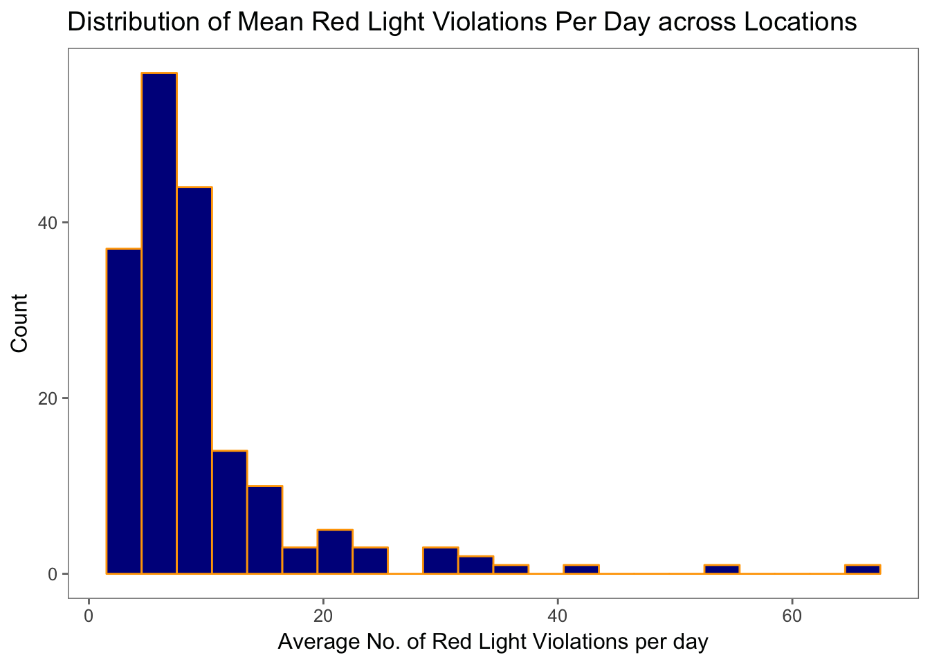
map <- ggmap(get_map(location = "chicago, illinois", zoom = 11, color = "bw")) +
  geom_point(data = loc_summary, aes(x = longitude,
                                     y = latitude,
                                     colour = log(avg_violations)),
             alpha = 1) +
  scale_colour_gradient(low = "lightyellow", high = "darkred",
                        name = "Log of Avg. Violations Per Day") +
  theme(axis.title.x = element_blank(),
        axis.text.x = element_blank(),
        axis.ticks.x = element_blank(),
        axis.ticks.y = element_blank(),
        axis.text.y = element_blank(),
        axis.title.y = element_blank(),
        legend.position = "top")

map
As shown above, the intersection at Cicero and I55 shows the darkest shade of red (65.47 violations per day on average). Let’s add some text labels for the top 5 intersections by average number of violations to make this easier to see.
map +
  geom_label_repel(data = head(loc_summary, 5),
                   aes(x = longitude,
                       y = latitude,
                       label = intersection),
                   size = 2,
                   min.segment.length = 0)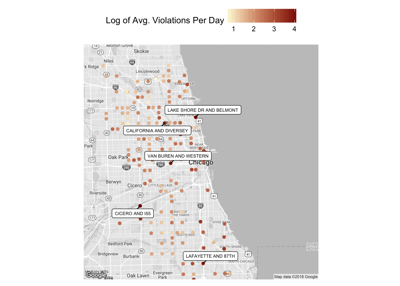
Finally, we’ll explore the time series properties of the daily count of total red light violations across the city of Chicago
Note that data from institutions around the world, many many more than just the City of Chicago, is available through Socrata.↩