
Analyzing My Google Fit Data
I’ve been using the Google Fit app to keep track of my fitness activity ever since I purchased my latest cell phone, around the end of 2017. I’ve found the app relatively easy to use; it provides plenty of options for a variety of different types of workouts, which is a bonus for me.
One thing I find lacking, however, is the ability to analyze/visualize fitness data within the app. Fortunately, fitness data is available for export to csv directly from your Google account. I found this help page useful. Included in the download is a file titled Daily Summaries.csv that contains a number of activites tracked by Google Fit, aggregated on a daily basis.
I was hoping to develop a more accessible picture of my fitness activity by using some tools readily available in R and the tidyverse.
library(tidyverse)
library(ggthemes)
library(tibbletime)
library(lubridate)
After finding the Daily Summaries.csv file in the download from Google, we can load into R and manipulate to our liking. Luckily, the csv is in a farily clean format already. In the code chunk below, we’re just doing some date formatting and renaming a few columns to be a bit less cumbersome.
# load data, format date variables
fit_data <- read.csv("~/kyle/Website/data/Daily Summaries.csv") %>%
  mutate(Date = as.Date(as.character(Date), format = "%Y-%m-%d")) %>%
  mutate(day = factor(weekdays(Date), levels = c("Sunday", "Monday", "Tuesday",
                                                 "Wednesday", "Thursday",
                                                 "Friday", "Saturday")),
         month = months(Date),
         year = year(Date)) %>%
  select(-Treadmill.walking.duration..ms.) %>%
  rename(n_steps = Step.count,
         n_calories = Calories..kcal.) %>%
  filter(Date > "2017-12-31") # 2018 only

# rename the activity duration columns to something less clunky
names(fit_data)[18:29] <- unlist(
  purrr::map(names(fit_data[, 18:29]),
                                       function(x){
                                         str_split(x, "\\.", n = 2)[[1]][1]
                                       })
)
Next, we’ll plot a time series of daily step totals. To smooth out some of the volatility, we can add the 7-day moving average of daily steps to the plot as well. Finally, we’ll add points to the observations where the 7-day moving average exceeds 10,000 steps to see when my goal of 10,000 steps is achieved more easily.
# function to compute moving average (from tibbletime package)
roll_mean_7 <- rollify(mean, window = 7)

# time series of daily step counts and calories burned, with 7-day moving average
ts_plot_data <- fit_data %>%
  select(Date, n_steps, n_calories) %>%
  mutate(ma_n_steps = roll_mean_7(n_steps),
         ma_n_calories = roll_mean_7(n_calories)) %>%
  gather(type, value, -Date)

ggplot(data = ts_plot_data %>% filter(type %in% c("n_steps", "ma_n_steps")),
       aes(x = Date, y = value, group = type, colour = type)) +
  geom_line(aes(alpha = type)) +
  geom_point(data = filter(ts_plot_data,
                           value >= 10000 & type == "ma_n_steps")) + # add points when 7-day MA over 10,000
  geom_line(aes(x = Date, y = 10000), colour = "black", linetype = 2,
            alpha = 0.3) +
  scale_alpha_manual(values = c(1, 0.5), guide = FALSE) +
  scale_colour_manual(values = c("orange", "darkblue"),
                      labels = c("7-day Moving Average",
                                 "N Steps"),
                      guide = guide_legend(reverse = TRUE)) +
  xlab("Date") +
  ylab("No. of Steps") +
  ggtitle("Daily Step Count") +
  theme_few() +
  theme(legend.title = element_blank(),
        legend.position = "bottom")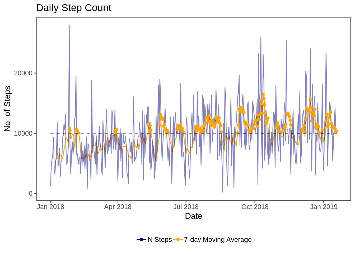
We can use the same procedure to investigate daily calorie burn over time:
ggplot(data = ts_plot_data %>% filter(type %in% c("n_calories", "ma_n_calories")),
       aes(x = Date, y = value, group = type, colour = type)) +
  geom_line(aes(alpha = type)) +
  geom_point(data = filter(ts_plot_data,
                           value >= 2700 & type == "ma_n_calories")) + # add points when 7-day MA over 2700
  geom_line(aes(x = Date, y = 2700), colour = "black", linetype = 2,
            alpha = 0.3) +
  scale_alpha_manual(values = c(1, 0.5), guide = FALSE) +
  scale_colour_manual(values = c("orange", "darkblue"),
                      labels = c("7-day Moving Average",
                                 "N Calories"),
                      guide = guide_legend(reverse = TRUE)) +
  xlab("Date") +
  ylab("No. of Calories") +
  ggtitle("Daily Calories Burned") +
  theme_few() +
  theme(legend.title = element_blank(),
        legend.position = "bottom")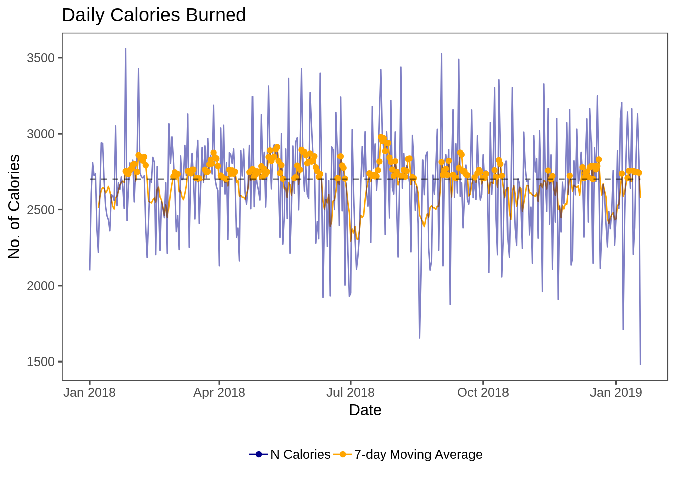
In the next chunk, we’ll look at the distribution of daily steps by day of the week (Sunday, Monday, etc.). Somewhat interestingly, my median daily step count is fairly constant across the week. The distribution of steps is the widest on the weekends, however (some very inactive Fridays, Saturdays, and Sundays, but some really active ones, too!).
# step count by day of the week
ggplot(data = fit_data,
       aes(x = day, y = n_steps)) +
  geom_boxplot(colour = "darkblue") +
  theme_few() +
  xlab("Day of Week") +
  ylab("Steps")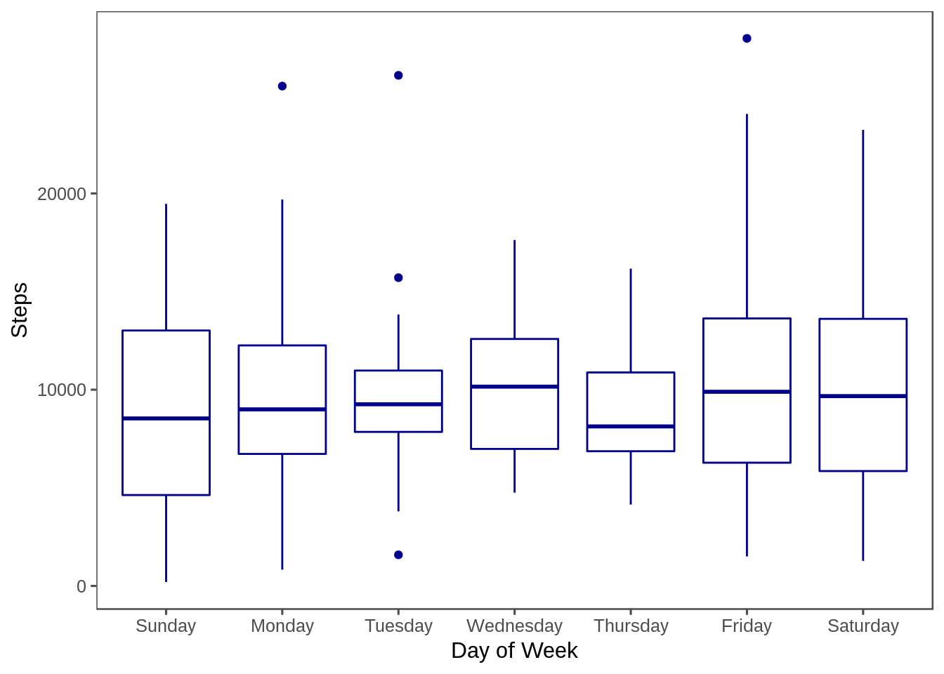
We’ll create an analagous plot for daily calories burned. A similar pattern emerges.
# inactivity by day of the week
ggplot(data = fit_data,
       aes(x = day, y = n_calories)) +
  geom_boxplot(colour = "darkblue") +
  theme_few() +
  xlab("Day of Week") +
  ylab("Calories Burned")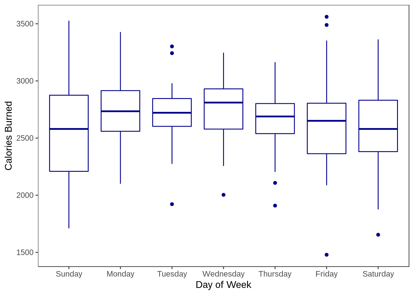
Finally, let’s look at the total amount of time spent performing different types of activities on a monthly basis. I think a bar chart is the most helpful way to visualize.
# bar plot of average monthly hours of activity by activity type
mnth_plot_data <- fit_data %>%
  #filter(as.Date(Date) > "2017-12-31") %>%
  #filter(month != "December") %>% # december not a complete month
  select(Date, Walking, Running, Basketball, Calisthenics,
         Elliptical, Golf, Weight, Treadmill, High) %>%
  rename(`Weight Lifting` = Weight,
         HIIT = High) %>%
  mutate(yr_month = as.Date(cut(Date, breaks = "month"))) %>%
  gather(type, value, -yr_month) %>%
  group_by(type, yr_month) %>%
  summarise(total_hrs = sum(value/3600000, na.rm = TRUE))

ggplot(data = mnth_plot_data,
       aes(x = yr_month,
           y = total_hrs, fill = type,
             label = round(total_hrs, 1))) +
    geom_bar(stat = "identity") +
    theme_few() +
    theme(axis.text.x = element_text(angle = 45))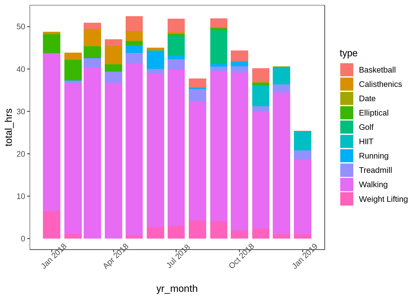
Walking makes up a significant chunk of my total activity time. Let’s look at the same chart, this time with walking removed.
ggplot(data = mnth_plot_data %>% filter(type != "Walking"),
       aes(x = yr_month, y = total_hrs, fill = type,
             label = round(total_hrs, 1))) +
    geom_bar(stat = "identity") +
    theme_few() +
    theme(axis.text.x = element_text(angle = 45))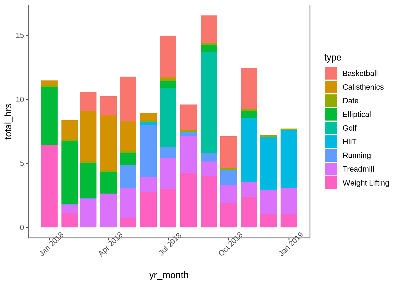
Moral of the story: not enough golf! :)